This is an Excel sheet that takes in several stocks, computes the returns and variations for portfolios created from them, and assembles all of this information into a graph of the CML and the Efficient Frontier. I created this sheet in the process of helping Wake Forest students prepare for a presentation. I’m storing it here in case I need it for another student or class.

It can be useful to demonstrate how correlation between multiple stocks affects the optimal weight that we should assign to different stocks. For example, a stock might have a low return but be negatively correlated with a riskier stock. This lower return stock would then act to reduce the risk of the overall portfolio.

Swapping out stocks with different relationships allows us to see how the tangent portfolio will ‘leverage’ their relationships to achieve an optimal Sharpe ratio.

Note: The CHOOSE function is used to create an array out of calculated portfolio weights within the formula rather than assemble those weights into separate visible arrays for each row of computation. This reduces visual clutter.

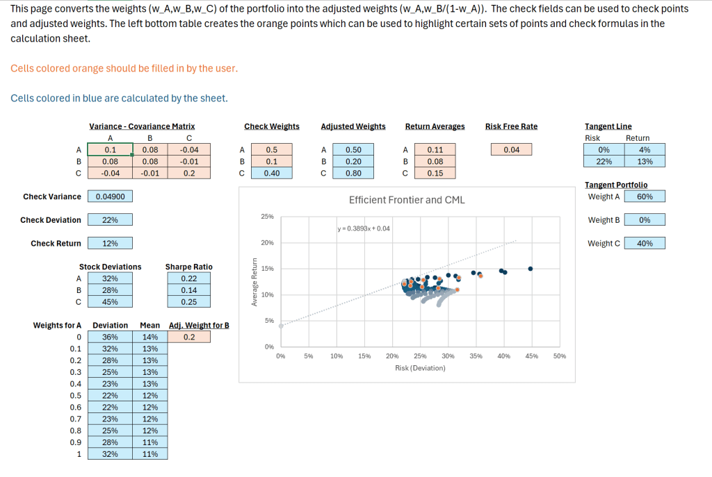
If you would like to play around with this sheet, you will need to download your own copy. If you wish to see the formulas that are used, you will need to unlock the sheets with the password 123. This password was used to lock blue cells that users don’t need to edit into order to use the sheet. This prevents errors from being introduced into the formulas of a working copy.

Broadly speaking, this sheet uses this formula

to calculate the deviations of a wide sample of portfolio weights. It also computes the expected returns of these portfolios using linearity of expectation.

It then graphs those points, computes their Sharpe ratios, uses XLOOKUP to find the portfolio with the highest Sharpe ratio, and then graphs the CML using that point and the risk-free return.

> Excel Functions Used:

XLOOKUP

“Use the XLOOKUP function to find things in a table or range by row. For example, look up the price of an automotive part by the part number, or find an employee name based on their employee ID. With XLOOKUP, you can look in one column for a search term and return a result from the same row in another column, regardless of which side the return column is on.” – Microsoft Support

MMULT

“The MMULT function returns the matrix product of two arrays. The result is an array with the same number of rows as array1 and the same number of columns as array2.” – Microsoft Support

TRANSPOSE

“Sometimes you need to switch or rotate cells. You can do this by copying, pasting, and using the Transpose option. But doing that creates duplicated data. If you don’t want that, you can type a formula instead using the TRANSPOSE function. For example, in the following picture the formula = TRANSPOSE(A1:B4) takes the cells A1 through B4 and arranges them horizontally.” – Microsoft Support

CHOOSE

“Uses index_num to return a value from the list of value arguments. Use CHOOSE to select one of up to 254 values based on the index number. For example, if value1 through value7 are the days of the week, CHOOSE returns one of the days when a number between 1 and 7 is used as index_num.” – Microsoft Support